Interested in this project?
Continue LearningLinear algebra is essential to machine learning. By identifying relationships of points in vector space, patterns can be determined that can lead to accurate predictions.
In this tutorial, we'll be calculating a best-fit line and using the equation of that line to model the linear relationship between the independent and dependent variables. In simpler terms, we'll be finding an equation to represent the correlations present in our dataset.
Linear regression is one of the simplest algorithms used in machine learning, and therefore it's good to start here.
Getting Started
First, we'll need to numpy. Then, let's define our x_values and y_values with some sample data.
import numpy as np

x_values = np.array([1,2,3,4,5,6,7,8,9,10])
y_values = np.array([1,4,1,6,4,7,4,6,10,8])
At the heart of linear algebra, we have the linear equation in slope-intercept form:
y = mx + b
However, what does this mean? This equation describes the linear relationship between x and y, with m being our slope and b being our y-intercept. In machine learning, our y value is the predicted label, b is the bias, the slope m is the weight, and the x value is a feature (input). You'll see these terms as you delve further into machine learning, such as in the Stock Price Prediction and Neural Network projects.
To determine our best-fit line, we first must start with the slope. The slope m of the best-fit line is defined as the following:
m = (( x̅ * y̅) - x̅y̅) / ( (x̅)²-(x̅²) )
In this equation, the over-line represents that we are taking the mean/average of the indicated values.
To find the y-intercept of our best fit line, we can do the following:
b = y̅ - mx̅
Programming Line of Best Fit
Now that we have the equations necessary to construct our best-fit line, let's get to coding it! Let's define our best_fit_line function which takes in the x and y values as parameters and returns the m and b values:
def best_fit_line(x_values,y_values):
    m = (((x_values.mean() * y_values.mean()) - (x_values * y_values).mean() ) /
         ( (x_values.mean()) ** 2 - (x_values ** 2 ).mean() ))

    b = y_values.mean() - m * x_values.mean()

    return m, b
Now that we have our slope and y-intercept values, we can construct an equation:
print(f"regression line: y = {round(m,2)}x + {round(b,2)}")

# output: y = 0.77x + 0.87
Here's a tip: the
fin front of the string creates a formatted string and allows us to interpolate values that might not even be strings!
Predictions
If we would like to make a prediction, we can do so by just passing in an input to our equation. Here's an example if we wanted to predict the output with an input (x) of 15:
x_prediction = 15
y_prediction = (m * x_prediction)+b
print(f"predicted coordinate: ({round(x_prediction,2)}, {round(y_prediction,2)})")

# output: (15, 12.41)
There you have it - a fully functioning linear regression model!
R Squared Value
Even though we have a linear model, it's not possible for it to be 100% accurate as we have a lot of variation in our data. The line of best fit simply finds the best representation of all the data points. The r^2 value, or coefficient of determination, allows us to numerically represent how good our linear model actually is. The closer the value is to one, the better the fit of the regression line. If the r^2 value is one, the model explains all the variability of the data.
The r^2 value is defined as the following:
r^2 = 1 - ((Squared Error of Regression Line) / (Squared Error of y Mean Line))
In this equation, we are dividing the square error of the regression line (sum of distances between regression line y values and original data y values squared) by the square error of the y mean line (sum of distances between y mean line y values and original data y values squared) and subtracting that value from one. The y mean line is a horizontal line at the mean of all the original y values. For example, if mean of the y_values was 5, the line would be at y = 5. In addition, the reason we square errors is to normalize the error values to be positive and punish for outliers (data points that do not follow the linear correlation).
Here's how we would implement this:
# y values of regression line
regression_line = [(m*x)+b for x in x_values]

def squared_error(ys_orig, ys_line):
    return sum((ys_line - ys_orig) * (ys_line - ys_orig)) # helper function to return the sum of the distances between the two y values squared

def r_squared_value(ys_orig,ys_line):
    squared_error_regr = squared_error(ys_orig, ys_line) # squared error of regression line
    y_mean_line = [mean(ys_orig) for y in ys_orig] # horizontal line (mean of y values)
    squared_error_y_mean = squared_error(ys_orig, y_mean_line) # squared error of the y mean line
    return 1 - (squared_error_regr/squared_error_y_mean)

r_squared = r_squared_value(y_values, regression_line)
print(f"r^2 value: {round(r_squared,2)}")
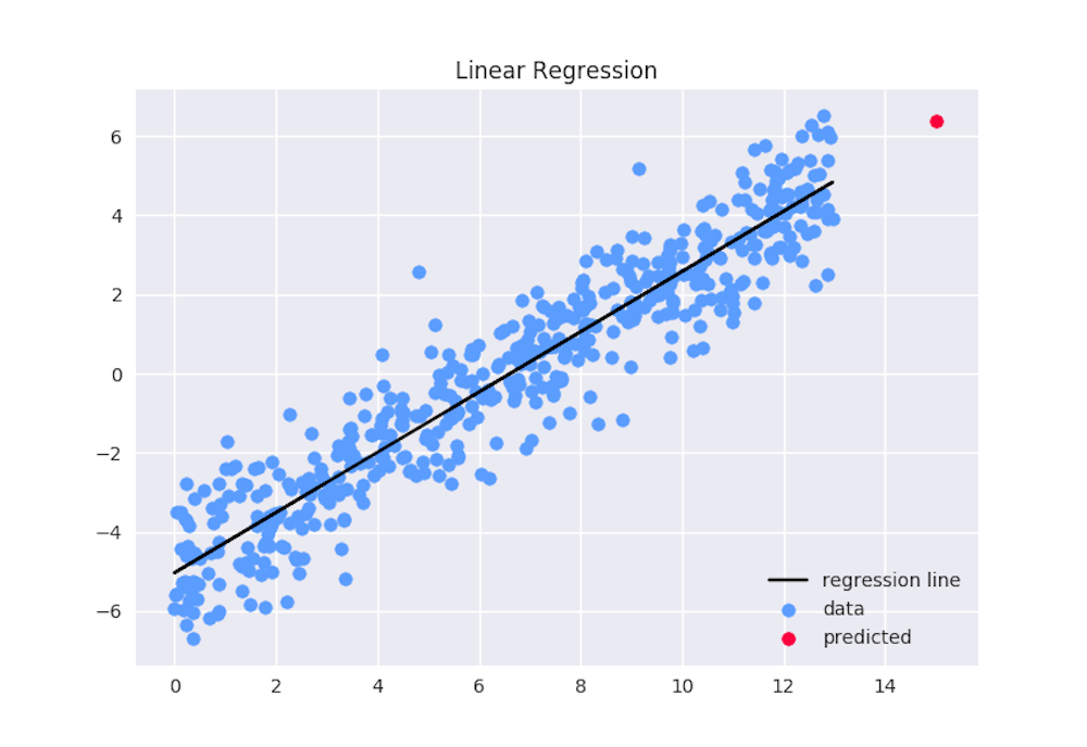
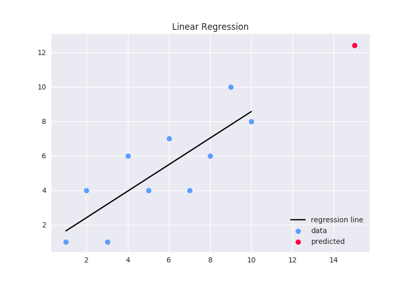
Plotting
To plot our points, regression line, and predicted output, we can use the matplotlib library:
import matplotlib.pyplot as plt

plt.title('Linear Regression')
plt.scatter(x_values, y_values,color='#5b9dff',label='data')
plt.scatter(x_prediction, y_prediction, color='#fc003f', label="predicted")
plt.plot(x_values, regression_line, color='000000', label='regression line')
plt.legend(loc=4)
plt.savefig("graph.png")
If you're doing this on Windows and not in a notebook environment, the UI with the graph won't pop up, but if you run the file in a Python Interactive Window, a file called
graph.pngshould be saved in the same folder as the python file!
There you go! Try using an actual dataset, such as housing or stock prices, and come up with a prediction!
Note: A traditional machine learning approach would be to use a gradient descent algorithm that iterates and adjusts the m and b values to minimize the loss (error) accordingly and arrive at the ideal equation. Gradient descent is used throughout machine learning and will be introduced in the Neural Network tutorial, but if you're interested, you can check out a video tutorial on linear regression using gradient descent here.
Be sure to move on to the other Machine Learning tutorials to learn more!
Comments (0)