Build a Random Forest Algorithm

Introduction

Thanks to libraries such as Scikit-Learn, it's now extremely easy to implement any machine learning algorithm in Python. It's so easy in fact, that often we don't need any underlying knowledge of how the model works under the hood in order to use it. While knowing all the details is not necessary, it's still helpful to have an idea of how the model trains and makes predictions. This lets us diagnose the model if performance is not as good as expected, or explain how our model makes decisions which is crucial when we want to convince others to use our models.

In this article, we'll look at how to build and use the Random Forest in Python, but rather than just show the code, we'll try to get an understanding of how the model works. We'll begin with a single decision tree on a simple problem, and then work our way to a complete random forest on a real-world data science problem. The complete code for this article is available as a Jupyter Notebook on GitHub.

Understanding a Decision Tree

A decision tree is the building block of a random forest and by itself is a rather intuitive model. We can think of decision trees as a flowchart of questions asked about our data, eventually leading to a predicted class (or continuous value in the case of regression). This is an interpretable model because it makes decisions how we do in real life: we ask a series of questions about the data until we eventually have arrived at a decision.

The main technical details of a decision tree are in how the questions about the data are constructed. A decision tree is built by forming questions that lead to the greatest reduction in Gini Impurity.

We'll get into Gini Impurity a little later, but what this means is that the decision tree tries to form nodes that are as pure as possible, containing a high proportion of samples (data points) from only one class.

Gini Impurity and constructing the tree may be a little tough to understand, so first let's build a Decision Tree, and then we can work through some simple math.

Decision Tree on a Simple Problem

We'll start with a very simple binary classification problem as shown below:

Our data only has two features (predictor variables) and there are a total of 6 data points with 2 different labels.

Although this problem is simple, it's not linearly separable, which means that we can't draw a single straight line through the data to classify the points. We can however draw a series of straight lines that divide the classes, which is essentially what the decision tree will do as it forms the series of questions.

To create the decision tree and train (fit) it on the data, we can use Scikit-Learn:

from sklearn.tree import DecisionTreeClassifier

# Make a decision tree and train

tree = DecisionTreeClassifier(random_state=RSEED)
tree.fit(X, y)

That's all there is to it!

During training we give the model both the features and the labels so it can learn to classify points based on the features. We don't have a testing set for this simple problem, but when testing, we only give the model the features and have it make predictions about the labels.

We can test the accuracy of our model on the training data:

print(f'Model Accuracy: {tree.score(X, y)}')

Model Accuracy: 1.0

We see that it gets 100% correct, which is what we expect because we gave it the answers (y) for training.

Visualizing a Decision Tree

So what's actually going on when we make a decision tree? I find the most helpful way to understand the decision tree is by visualizing it, which we can do using a Scikit-Learn utility (for details check out the notebook or this article).

This shows the entire structure of the decision tree. All the nodes, except for the leaf nodes (terminal nodes), have 5 parts:

1. Question asked about the data based on a value of a feature. Each question has either a True or False answer.
   Based on the answer to the question, a data point moves through the tree.
2. gini: The Gini Impurity of the node. The average weighted Gini Impurity must decrease
   as we move down the tree.
3. samples: The number of observations in the node.
4. value: The number of samples in each class. For example, the top node has 2 samples in
   class 0 and 4 samples in class 1.
5. class: The majority classification for points in the node (defaults to 0 for ties). In the case
   of leaf nodes, this is the prediction for all samples in the node.

The leaf nodes do not have a question because these are where the final predictions are made. To classify a new point, simply move down the tree, using the features of the point to answer the questions until you arrive at a leaf node where the class is the prediction of the tree. You can try it out using the points above or test out different predictions in the notebook.

Gini Impurity

At this point we should try to understand the Gini Impurity. Put simply, the Gini Impurity is the probability that a randomly chosen sample in a node would be incorrectly labeled if it was labeled by the distribution of samples in the node. For example, in the top (root) node, there is a 44.4% chance of incorrectly classifying a data point chosen at random based on the distribution of sample labels in the node.

The Gini Impurity is how the decision tree decides the feature values on which to split a node (the question asked about the data). The tree searches through all the features for the split resulting in the maximum reduction in impurity.

An impurity of 0 is perfect because that means there is no chance a randomly selected sample would be incorrectly labeled and this can only occur when all the samples in a node are from the same class! At each level of the tree, the weighted average gini impurity decreases, indicating the nodes become more pure (An alternative for splitting nodes is using the information gain, a related concept).

The equation for Gini Impurity of one node is:

where p_i is the fraction of points in class i in the node. Let's walk through calculating the Gini Impurity of the root (top) node.

Out of this very simple math, a very powerful machine learning model emerges!

This is the total Gini Impurity for the top level of the tree since there is only the root node. At the second layer of the tree, the leftmost node has 0.5 Gini Impurity which seems to suggest an increase in the impurity. However, it's the weighted average of the Gini Impurity which decreases at each level. Each node is weighted by the fraction of samples from the parent node that are in that node. So the overall Gini Impurity for the second level is:

As we move down the tree, the nodes get more and more pure until eventually, at the final layer, the Gini Impurity has reached 0.0, indicating each node contains only samples from one class. This is as expected because we did not limit the depth of the tree and allowed it to create as many levels as necessary in order to classify all points. Although our model correctly classified all training points, this does not mean it is perfect, because it is likely overfitting to the training data.

Overfitting: why a forest is better than one tree

You might be tempted to ask why not just use one decision tree? It seems like the perfect classifier since it did not make any mistakes! A critical point to remember is that the tree made no mistakes on the training data.

We expect this to be the case since we gave the tree the answers. The point of a machine learning model is to generalize well to the testing data. Unfortunately, when we do not limit the depth of our decision tree, it tends to overfit to the training data.

Overfitting occurs when our model has high variance and essentially memorizes the training data. This means it can do very well - even perfectly - on the training data, but then it will not be able to make accurate predictions on the test data because the test data is different! What we want is a model that learns the training data well, but then also can translate that to the testing data. The reason the decision tree is prone to overfitting when we don't limit the maximum depth is because it has unlimited complexity, meaning that it can keep growing until it has exactly one leaf node for every single observation, perfectly classifying all of them.

To understand why a decision tree has high variance, we can think of it in terms of a single person. Imagine you have to decide whether Apple stock will go up tomorrow and you decide to ask a few analysts. Any one analyst is likely to have high variance and will rely strongly on the data which they have access to - one analyst might read only pro-Apple news and hence she thinks the price can go up, while the other has recently heard from her friends that Apple products have started to decrease in quality and she thinks the price is due for a downturn. These individual analysts have high variance because their answers are extremely dependent on the data they have seen.

Instead of asking individual analysts, we could poll an entire roomful of experts, and make the final decision based on the most common answer. Because each analyst has access to different data, we would expect individual variance to be high, but the overall variance of the entire ensemble should be reduced. Using many individuals is essentially the idea behind a random forest: rather than one decision tree, use hundreds or thousands to form a powerful model. The final prediction from the model then becomes the average prediction from all trees in the ensemble. (The problem of overfitting is known as the bias-variance tradeoff and is a fundamental topic in machine learning).

Random Forest

The random forest is a model made up of many decision trees. Rather than just being a forest though, this model is random because of two concepts:

1. Random sampling of data points
2. Splitting nodes based on subsets of features

Random Sampling

One of the keys behind the random forest is that each tree trains on random samples of the data points. The samples are drawn with replacement (known as bootstrapping) which means that some samples will be trained on in a single tree multiple times (we can also disable this behavior if we want). The idea is that by training each tree on different samples, although each tree might have high variance with respect to a particular set of the training data, overall, the entire forest will have low variance. This procedure of training each individual learner on different subsets of the data and then averaging the predictions
is known as bagging, short for bootstrap aggregating.

Random Subsets of Features

Another concept behind the random forest is that only a subset of all the features are considered for splitting each node in each decision tree. Generally this is set to sqrt(n_features) meaning that at each node, the decision tree considers splitting on a sample of the features totaling the square root of the total number of features. The random forest can also be trained considering all the features at every node. (These options can be controlled in the Scikit-Learn random forest implementation).

If you grasp a single decision tree, bagging decision trees, and random subsets of features, then you have a pretty good understanding of how a random forest works. The random forest combines hundreds or thousands of decision trees, trains each one on a slightly different set of the observations (sampling the data points with replacement) and also splits nodes in each tree considering only a limited number of the features. The final predictions made by the random forest are made by averaging the predictions of each individual tree.

Random Forest in Practice

Much like any other Scikit-Learn model, to use the random forest in Python requires only a few lines of code. We'll build a random forest, but not for the simple problem presented above. To contrast the ability of the random forest with a single decision tree, we'll use a real-world dataset split into a training and testing set.

Dataset

The problem we'll solve is a binary classification task. The features are socioeconomic and lifestyle characteristics of individuals and the label is 0 for poor health and 1 for good health. This dataset was collected by the Centers for Disease Control and Prevention and is available here. This is an imbalanced classification problem, so accuracy is not an appropriate metric. Instead we'll measure the Receiver Operating Characteristic Area Under the Curve (ROC AUC), a measure from 0 (worst) to 1 (best) with a random guess scoring 0.5. We can also plot the ROC curve to assess the models performance.

The notebook contains the implementation for both the decision tree and the random forest, but here we'll just focus on the random forest. After reading in the data, we can instantiate and train a random forest as follows:

from sklearn.ensemble import RandomForestClassifier

# Create the model with 100 trees

model = RandomForestClassifier(n_estimators=100,
random_state=RSEED,
max_features = 'sqrt',
n_jobs=-1, verbose = 1)

# Fit on training data

model.fit(train, train_labels)

After a few minutes to train, the model is ready to make predictions on the testing data as follows:

rf_predictions = model.predict(test) rf_probs = model.predict_proba(test)[:, 1]

We make class predictions (predict) as well as predicted probabilities (predict_proba) which are needed to calculate the ROC AUC. Once we have the testing predictions, we can compare them to the testing labels
to calculate the ROC AUC.

from sklearn.metrics import roc_auc_score

# Calculate roc auc

roc_value = roc_auc_score(test_labels, rf_probs)

Results

The final ROC AUC for the random forest was 0.87 compared to 0.67 for the single decision tree. If we look at the training scores, we notice that both models achieved 1.0 ROC AUC, which again is as expected because we gave these models the training answers and did not limit the maximum depth. However, although the random forest overfits, it is able to generalize much better to the testing data than the single decision tree.

If we inspect the models, we see that the single decision tree reached a maximum depth of 55 with a total of 12327 nodes. The average decision tree in the random forest had a depth of 46 and 13396 nodes. Even with a larger average number of nodes, the random forest was better able to generalize!

We can also plot the ROC curve for the single decision tree (top) and the random forest (bottom). A curve to the top and left is a better model:

We see that the random forest significantly outperforms the single decision tree.

Another diagnostic measure of the model we can take is to plot the confusion matrix for the testing predictions (see the notebook for details):

Feature Importances

The feature importances in a random forest indicate the sum of the reduction in Gini Impurity over all the nodes that are split on that feature. We can use these to try and figure out what predictor variables the random forest considers most important. The feature importances can be extracted from a trained random forest and put into a Pandas dataframe as follows:

import pandas as pd

fi = pd.DataFrame({'feature': list(train.columns),
'importance': model.feature*importances*}).
sort_values('importance', ascending = False)

fi.head()

feature importance
tDIFFWALKt0.036200
tQLACTLM2t0.030694
tEMPLOY1t 0.024156
tDIFFALONt0.022699
tUSEEQUIPt0.016922
tDECIDEt 0.016271
t_LMTSCL1t0.013424
tINCOME2t 0.011929
tCHCCOPD1t0.011506
t_BMI5t 0.011497

We can also use the feature importances for feature selection by removing features with 0 or low importance.

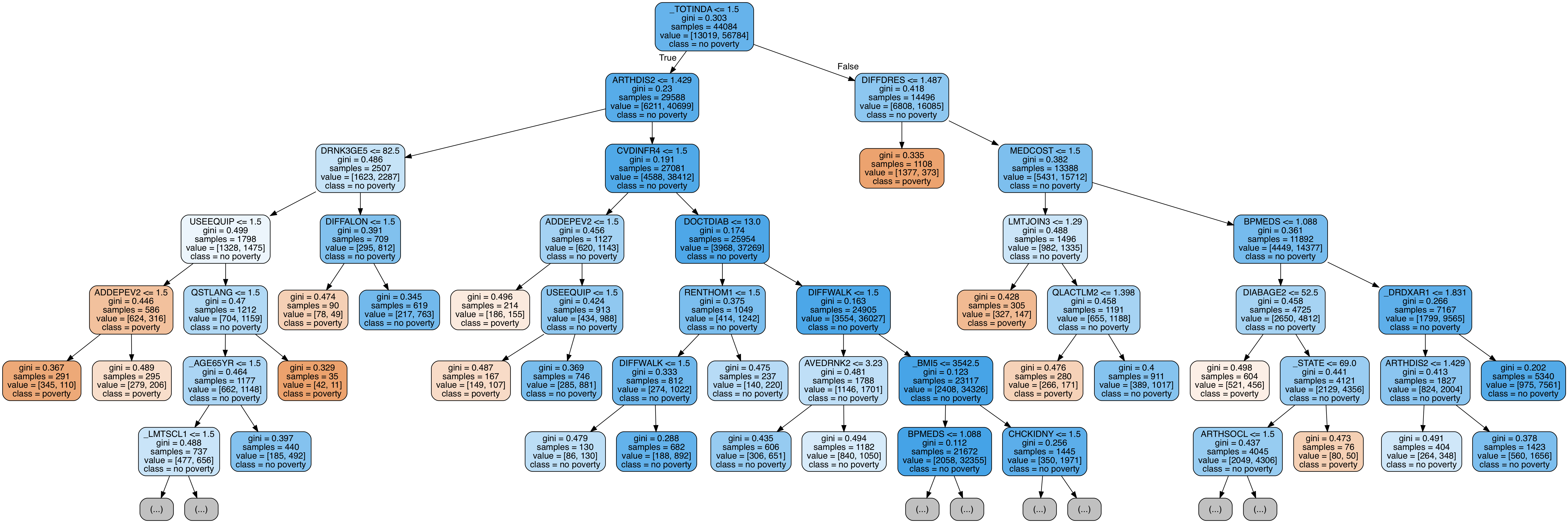
Visualize Tree in Forest

Finally, we can visualize a single decision tree in the forest. This time, we have to limit the depth of the tree otherwise it will be too large to be converted into an image. To make the figure below, I limited the maximum depth to 6. This still results in a large tree that we can't completely parse!

Next Steps

One potential next step is to optimize the random forest which we can do via random search and the RandomizedSearchCV in Scikit-Learn..

Optimization refers to finding the best hyperparameters fior a model on a given dataset. The best hyperparameters will vary between datasets, so we have to perform optimization (also called model tuning) separately on each datasets. I like to think of model tuning as finding the best settings for a machine learning algorithm.

For an implementation of random search for model optimization of the random forest, refer to the Jupyter Notebook.

Conclusions

While we can build powerful machine learning models without understanding anything about them, it's far more useful to at least have some knowledge about what is occurring under the hood. In this article, we not only built and used a random forest in Python, but we also developed an understanding of the model.

We first looked at an individual decision tree, the basic building block of a random forest, and then we saw how we can combine hundreds of decision trees in an ensemble model. This ensemble model, when used with bagging and random sampling of features, is called a random forest. The key concepts to understand from this article are:

1. Decision tree: intuitive model that makes decisions based on a flowchart of questions asked about feature values. Has high variance indicated by overfitting to the training data.
2. Gini Impurity: Measure that the decision tree tries to minimize when splitting each node. Represents the probability that a randomly selected sample from a node will be incorreclty classified according to the distribution of samples in the node.
3. Bootstrapping: sampling random sets of observations with replacement. Method used by the random forest for training each decision tree.
4. Random subsets of features: selecting a random set of the features when considering how to split each node in a decision tree.
5. Random Forest: ensemble model made of hundreds or thousands of decision trees using bootstrapping, random subsets of features, and average voting to make predictions. This is an example of a bagging ensemble.
6. Bias-variance tradeoff: the fundamental issue in machine learning that describes the tradeoff between a model with high complexity that learns the training data very well at the cost of not being able to generalize to the testing data (high variance), and a simple model (high bias) that cannot even learn the training data. A random forest reduces the variance of a single decision tree while also accurately learning the training data leading to better predictions on the testing data.

Hopefully this article has given you the confidence and understanding needed for you to start using the random forest on your projects. The random forest is a powerful machine learning model, but that should not prevent us from knowing how it works! The more we know about a model, the better equipped we will be to use it effectively and explain how it makes predictions so others will trust it! Now get out there and solve some problems with the random forest.