Interested in this project?
Continue LearningPredicting the Market
In this tutorial, we'll be exploring how we can use Linear Regression to predict stock prices thirty days into the future. You probably won't get rich with this algorithm, but I still think it is super cool to watch your computer predict the price of your favorite stocks.
Getting Started
Create a new stock.py file. In our project, we'll need to import a few dependencies. If you don't have them installed, you will have to run pip install [dependency] on the command line.
import quandl
import pandas as pd
import numpy as np
import datetime

from sklearn.linear_model import LinearRegression
from sklearn import preprocessing, svm
from sklearn.model_selection import train_test_split
We are using Quandl for our stock data, pandas for our dataframe, numpy for array and math fucntions, and sklearn for the regression algorithm.
Stock Data & Dataframe
To get our stock data, we can set our dataframe to quandl.get("WIKI/[NAME OF STOCK]"). In this tutorial, I will use Amazon, but you can choose any stock you wish.
df = quandl.get("WIKI/AMZN")
If we print(df.tail()) and run our python program, we see that we get a lot of data for each stock:
Open     High      Low    Close     Volume  Ex-Dividend  \
Date
2017-12-13  1170.00  1170.87  1160.27  1164.13  2555053.0          0.0
2017-12-14  1163.71  1177.93  1162.45  1174.26  3069993.0          0.0
2017-12-15  1179.03  1182.75  1169.33  1179.14  4539895.0          0.0
2017-12-18  1187.37  1194.78  1180.91  1190.58  2767271.0          0.0
2017-12-19  1189.15  1192.97  1179.14  1187.38  2555235.0          0.0

Split Ratio  Adj. Open  Adj. High  Adj. Low  Adj. Close  \
Date
2017-12-13          1.0    1170.00    1170.87   1160.27     1164.13
2017-12-14          1.0    1163.71    1177.93   1162.45     1174.26
2017-12-15          1.0    1179.03    1182.75   1169.33     1179.14
2017-12-18          1.0    1187.37    1194.78   1180.91     1190.58
2017-12-19          1.0    1189.15    1192.97   1179.14     1187.38

Adj. Volume
Date
2017-12-13    2555053.0
2017-12-14    3069993.0
2017-12-15    4539895.0
2017-12-18    2767271.0
2017-12-19    2555235.0
However, in our case, we only need the Adj. Close column for our predictions.
df = df[['Adj. Close']]
Now, let’s set up our forecasting. We want to predict 30 days into the future, so we’ll set a variable forecast_out equal to that. Then, we need to create a new column in our dataframe which serves as our label, which, in machine learning, is known as our output. To fill our output data with data to be trained upon, we will set our prediction column equal to our Adj. Close column, but shifted 30 units up.
forecast_out = int(30) # predicting 30 days into future
df['Prediction'] = df[['Adj. Close']].shift(-forecast_out) #  label column with data shifted 30 units up
You can see the new dataframe by printing it: print(df.tail())
Defining Features & Labels
Our X will be an array consisting of our Adj. Close values, and so we want to drop the Prediction column. We also want to scale our input values. Scaling our features allow us to normalize the data.
X = np.array(df.drop(['Prediction'], 1))
X = preprocessing.scale(X)
Now, if you printed the dataframe after we created the Prediction column, you saw that for the last 30 days, there were NaNs, or no label data. We’ll set a new input variable to these days and remove them from the X array.
X_forecast = X[-forecast_out:] # set X_forecast equal to last 30
X = X[:-forecast_out] # remove last 30 from X
To define our y, or output, we will set it equal to our array of the Prediction values and remove the last 30 days where we don’t have any pricing data.
y = np.array(df['Prediction'])
y = y[:-forecast_out]
Linear Regression
Finally, prediction time! First, we’ll want to split our testing and training data sets, and set our test_size equal to 20% of the data. The training set contains our known outputs, or prices, that our model learns on, and our test dataset is to test our model's predictions based on what it learned from the training set.
X_train, X_test, y_train, y_test = train_test_split(X, y, test_size = 0.2)
Now, we can initiate our Linear Regression model and fit it with training data. After training, to test the accuracy of the model, we "score" it using the testing data. We can get an r^2 (coefficient of determination) reading based on how far the predicted price was compared to the actual price in the test data set. When I ran the algorithm, I usually got a value of over 90%.
# Training
clf = LinearRegression()
clf.fit(X_train,y_train)
# Testing
confidence = clf.score(X_test, y_test)
print("confidence: ", confidence)
Lastly, we can to predict our X_forecast values:
forecast_prediction = clf.predict(X_forecast)
print(forecast_prediction)
Here's what I got for AMZN stock (12/19/17):
('confidence: ', 0.989032635604704)
[ 1163.89768621  1166.50500319  1172.69608254  1168.7695255   1172.7376334
  1180.70501237  1170.16147958  1181.17245963  1173.47516131  1169.76674633
  1183.45775738  1200.77408167  1231.77102929  1241.98215513  1239.66569423
  1206.08220507  1222.16239103  1207.20407851  1177.70296214  1185.61840252
  1196.81636148  1204.54482295  1206.84050841  1214.0288086   1210.03992526
  1209.05309214  1219.57584949  1224.6450554   1236.52860369  1233.20453424]
What's next?
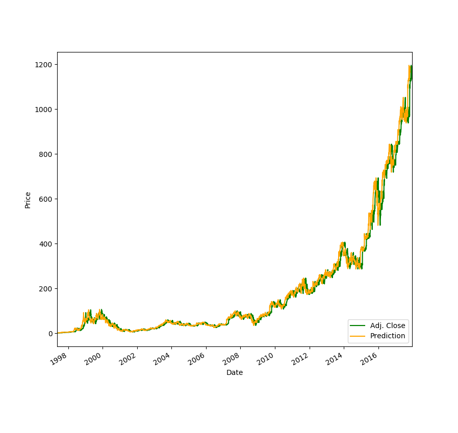
Try and plot your data using matplotlib. Make your predictions more advanced by including more features. When completed, feel free to share your projects in the comments! I'd love to check them out :)
Comments (0)