Interested in this project?

Introduction

Tutorial Dependencies

Before you start this tutorial, it is essential that you are aware of basic Python syntax to ensure you understand this exploration. Also, make sure to view the Linear Regression tutorial on Enlight as it helps with an understanding of Logistic Regression.

Linear Regression Tutorial

Nonetheless, if you aren't there, don't worry as we will do our best to ensure you understand all the concepts discussed in this tutorial. Before we create a Logistic Regression algorithm, let's understand what it is!

Understanding Logistic Regression and the Problem

To start, we need to understand the problem and what we are trying to find. In a football match, there are three possible outcomes for a team: a win, a draw, or a loss. In every game, there is a home team and an away team. In this tutorial, we will examine the likelihood of a home team winning a football match. This suggests we have a classification problem, where the variable we are trying to predict has discrete values. In this scenario, we are mainly predicting two unique outcomes: a home team winning the match or the home team not winning the match (home team draws or losses the match).

To explain Logistic Regression, I will use a simple example that has two outcomes. Based on someone's weight, can we predict if they are obese? In this scenario, there are two outcomes: obese or not obese. This outcome is determined by a feature: the person's weight. IIn this problem, the variable y we are trying to predict can be thought of as taking two values, either a 0 for not obese or a 1 for obese. This is known as a binary classification problem.

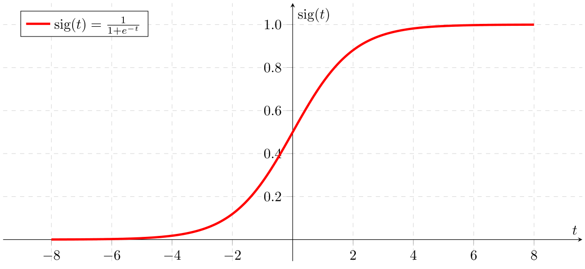
You might be wondering, can't we just use linear regression for this problem? Simply put, linear regression is useful when predicting an output with a continuous value, such as predicting the cost of renting a house in Boston based on its size. However, for classification problems, Logistic Regression predicts the probability between 0 and 1 for a specific outcome on a Sigmoid curve. Alt

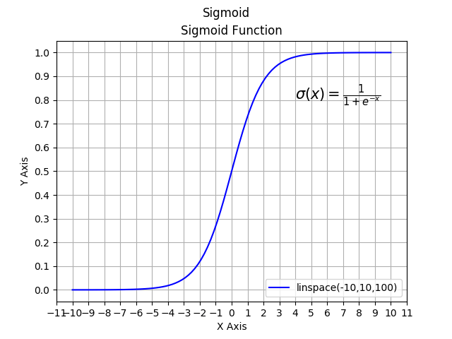
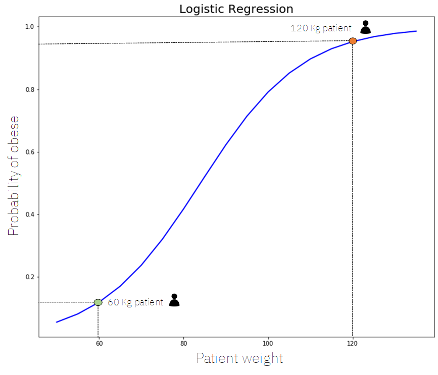
Let's examine this Sigmoid function. Firstly, we can see the range of the Y-axis from 0 to 1. Using the features, such as a person's weight, we can get the probability of a specific occurrence.

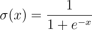
As seen in the graph, the formula for the sigmoid function is: Using this function, we need to calculate the probability. Let's understand what Logistic Regression does to calculate the probability. The Logistic Regression model needs to learn from the data. We can't expect it to "magically" predict the outcome. To ensure we get high accuracy, the model needs to learn from the training dataset. Typically, with any dataset in Machine Learning, it is split into a training and testing dataset. The training dataset helps improves the model, while the testing dataset validates the model's accuracy.

In the data, we have certain input features; in this simple example, we only have one input feature: the weight of the individual (kg). With machine learning models, there is an associated weight, a real number associated with the input feature (weight in kg) that represents how significant the input feature is to the decision to classify the individual as obese or not. In the example below, it is denoted by the greek symbol θ. It is particularly useful when you have more than one input feature, as the model may detect a strong correlation between an input feature and the classification decision, which would result in a greater θ value. However, if the model detects a weak correlation between an input feature and the classification decision, the input feature would have a lower θ value, or possibly a negative value! Another term included is a bias term c, which is a real number that is summed with the weighted input features.

To calculate the probability, we need to calculate the sum of the weighted inputs for the Sigmoid function:

However, we aren’t done yet. We need to train the model. You might be wondering, how are these weights exactly calculated? What method is used? Methods such as Gradient Descent are used to calculate the weights of the model.

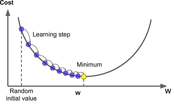
Gradient Descent is an algorithm that finds the minimum of a loss function. A loss function is used to evaluate a possible solution (value of the weights associated with the input features and the bias term). It starts at a random point on the function and moves in the negative direction of the gradient of the function to reach the minima. Its goal is to reach a gradient of zero, which occurs at the minimum. Here is a visual representation of the optimization algorithm: Source

For a detailed understanding of gradient descent, check out this video.

Let's explore the process of training a logistic regression model.

First, we require data of individuals who are obese and not obese, along with their weights in a file.
To train our model, we use the Gradient Descent algorithm in order to fit the outcomes to a Logistic Curve.
After training the model, we obtain the parameters of the model.
Now, we can make predictions using this equation and data. Let’s say we have two patients: one who weighs 60kg and another who weighs 120kg. If we put these inputs into the model, we can calculate the probability that the individual is obese and fit it on the Sigmoid curve.

After this, we can visualize these results on the Sigmoid curve. Source

Examining the earlier example, if an individual weighs 60kg, the probability that they are obese is approximately 0.12 (12%). However, if an individual weighs 120kg, the likelihood that they are obese is about 0.98 (98%).

Setting Up

Data & Libraries

To start, create a Python Notebook with a .ipynb extension on your favorite IDE! I recommend using Jupyter Notebooks or Google Colab. Before we start, we need to install a few libraries that allow us to analyze, manipulate, and visualize data. If you don’t have pandas, scikit-learn, or seaborn, you can install them with the following commands:

pip install pandas
pip install -U scikit-learn
pip install seaborn

If you're using Anaconda, type this in your conda environment (if you're not, just move on!): pandas is already installed if you use Anaconda.

conda install scikit-learn
conda install seaborn

For more assistance, visit these links:

Install pandas

Install scikit-learn

Install seaborn

Let’s start importing a few required libraries and add the magic function from IPython

import pandas as pd
%matplotlib inline #magic function to ensure we can plot on notebooks

After this, we need to download the dataset that will be analyzed in this tutorial. I gathered historical Premier League data from the 2000/01 season onwards and processed it to ensure it is easy to understand.

Download Data

Now, it is time to import our data as a pandas dataframe.

data = pd.read_csv('pl_dataset.csv')

If you have saved your .csv file in a different directory, you need to put the address. For example, I saved the data on my Desktop, so my code is:

data = pd.read_csv('C:/Users/salga/OneDrive/Desktop/data/pl_dataset.csv')

This data is still not perfect. We need to remove some columns from the dataframe that are unnecessary to predict if the home team will win. If you examine the dataset, you can see it includes columns that show the past results. Form plays a major role in predicting the outcome of a match. A team's form influences the team's morale and suggests a team in good form is usually predicted to win. As such, we will remove games in the first three matchweeks, as we require some past results to assist us in predicting if the home team will win the football match.

data_MW = data[data.MW > 3] #Ensures that games from the first three matchweeks are removed

data_MW will include matches after matchweek 3. data will include all the matches, including matches from matchweek 1, 2, and 3.

After this, we need to remove some unnecessary columns. Using .drop, we can some specific rows or columns.

data_MW.drop(['Unnamed: 0','HomeTeam', 'AwayTeam', 'Date', 'MW', 'HTFormPtsStr', 'ATFormPtsStr', 'FTHG', 'FTAG',
           'HTGS', 'ATGS', 'HTGC', 'ATGC','HomeTeamLP', 'AwayTeamLP','DiffPts','HTFormPts','ATFormPts',
           'HM4','HM5','AM4','AM5','HTLossStreak5','ATLossStreak5','HTWinStreak5','ATWinStreak5',
           'HTWinStreak3','HTLossStreak3','ATWinStreak3','ATLossStreak3'],1, inplace=True)

This code removes columns such as the name of specific teams, the date of the match, the matchweek, and their specific league positions. The data remaining already consists of most of the data: for instance, instead of including columns such as HomeTeamLP, which is the league position of the home team. The difference between the league position of the home team and away team is within the dataset. Many of the columns don't add value to the model, as they aren't integers, and are in different forms such as strings for the name of teams. The matchweek itself doesn't have a correlation to results as the Premier League randomizes matchups between teams.

To preview the data within the dataset, write the following code:

data_MW

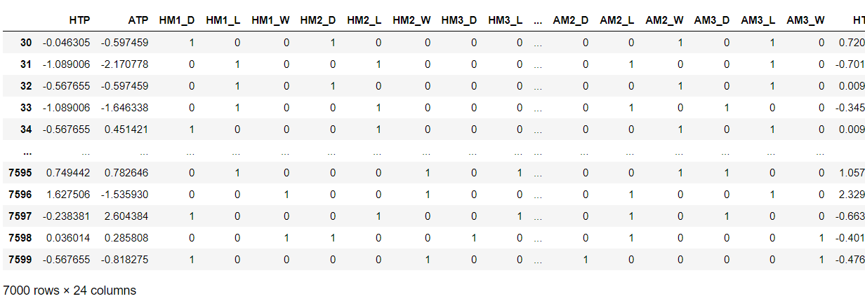
You should see the following output, which shows the first 5 rows and the last 5 rows within our dataset. 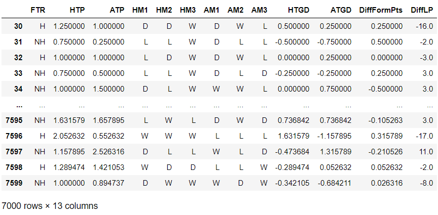Lets attempt to understand each column! FTR is the full-time result, which is either H for Home win or NH for Not Home win, which is either a draw or a loss for the home team. HTP is the home team average points, which aggregates the number of points and divides it by the matchweek. ATP works similarly to HTP but is the away team average points. HM1 is home match 1, which gives the result of the most recent game for the home team. This is similar to HM2, and HM3, which provides the 2nd most recent match and 3rd most recent match. AM1, AM2, and AM3 are the results of the away team. HTGD is the average goal difference for the home team, which calculates an average similar to how HTP works. ATGD is the average goal difference for the away team. DiffFormPts is the average difference in points between the two teams from the 5 last matches. DiffLP is the difference in the team's respective league positions from the previous football season.

Data Exploration

Since we are predicting if the home team wins or losses, let's calculate the percentage of matches won by the home team. First, we need to find the number of matches played from the 2000/01 Premier League season to the 2019/20 Premier League season. For this, let's use the data that includes all the matchweeks. To do so, write the following code:

no_of_matches = len(data.index)

First, we use len to get the number of rows in the pandas dataframe, which gives us the number of matches. Then, we need to find the number of matches won by the home team. To do so, write the following code:

no_of_homewins = len(data[data.FTR == 'H'])

This checks the FTRcolumn and counts the number of rows that satisfy the condition that the home team won. Finally, let's calculate the win rate for the home team:

win_pct = (no_of_homewins/no_of_matches) * 100

We calculate the proportion of home victories to the number of matches played and multiply the result by 100 to get a percentage. Now let's output the results!

print ("Number of matches: "+ str(no_of_matches)) #have to use str as integers and strings cannot be concatenated 
print ("Number of home victories: "+ str(no_of_homewins))
print ("Win Percentage: "+ str(round(win_pct,2))+"%") #round to 2dp

Out of 7600 matches, the home team won 3529 matches, resulting in a win percentage of approximately 46.4%. This means that the home team either drew or lost approximately 53.6% of their matches. This suggests that we can't just pick a winner based on if a team is playing at their home stadium.

Exercise: Data Exploration

Based on the example, can you find the percentage of matches in which the home team won and had a positive average goal difference?

Solution

no_of_matches = len(data.index)
no_of_homewins_withGD = len(data[(data.FTR == 'H') & (data.HTGD > 0)])
win_pct_GD = (no_of_homewins_withGD/no_of_matches) * 100

Data Visualization

Now, let’s try to find a correlation between some of the features included in the dataset. To do so, we can create a heatmap using seaborn, a data visualization library. First, let's import the seaborn library. With one line of code, we can create an extremely useful heatmap with annotations:

import seaborn as sns #data visualization
sns.heatmap(data_MW.corr(), annot=True) #here we use data because it only includes the necessary features

It outputs the following the heatmap: 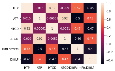Alt This heatmap shows a few correlations. For instance, the home average goal difference (HTGD) and the away average goal difference (ATGD) has a high correlation with the average home points (HTP) and average away points (ATP). A correlation of 0.92 exists, which suggests a very strong correlation between the input features. This logically makes sense because a team that performs well generally score more goals than their opposition and, hence, earn more points, and vice-versa.

Data Preparation

Now, we need to prepare the data before performing Logistic Regression. To start, we need to separate the features and the final output. The target, which is the FTR, needs to be assigned to a separate variable and removed from the variable the contains all of the features.

x_features = data_MW.drop(['FTR'],1) #remove FTR, where the ,1 indicates a column
y_target = data_MW['FTR'] #creates a variable with one column with all the full time results

Now, we need to standardize all the data. Standardization is imperative to the success of the machine learning model we create. Models may not behave as intended features do not have a normal distribution. As such, the scale method creates a Gaussian distribution with unit variance and zero mean.

In the x_features variable, there are 6 features that are integers. Since we do not want to standardize non-integers, we need to create an array of column labels, and then scale all the columns individually using a for loop. Before that, we import scale from the sklearn.preprocessing library.

from sklearn.preprocessing import scale #used to standardize data
columns = [['HTP','ATP','HTGD','ATGD','DiffFormPts','DiffLP']]
for column in columns:
    x_features[column] = scale(x_features[column])

Now, we are going to preprocess all the features before we train and evaluate the model. Categorical variables such as HM1, will be converted into numerical variables. This is known as one-hot encoding. As such, new columns will be created such as HM1_D, HM1_L, and HM1_W, and each will be assigned with either a 0 or a 1. It will be a 1, if HM1, was that specific column label, and a 0 if not. For instance, if HM1 for a specific team was W, then HM1_D = 0, HM1_L = 0 and HM1_W = 1. Here is an example: 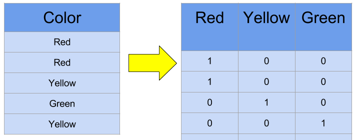Source

To do so, we will start by creating a new pandas dataframe, that will consist of the modified features with additional columns.

plDF = pd.DataFrame(index = x_features.index) #sets the index - rows from 30 onwards.

This creates a dataframe without any column data but rather the rows included in the dataframe. After this, we use the .join method to join the column data to the specific rows.

Then, we iterate through each feature and check if each feature is categorical. If categorical, it needs to be converted into a continuous variable (indicators).

for column, column_data in x_features.iteritems(): #iteritems iterates through each column

    if column_data.dtype == object: ## an object is not an integer
            column_data = pd.get_dummies(column_data, prefix = column) #converts into indicator 
            
    plDF = plDF.join(column_data) #joins each column and puts it on dataframe

x_features = plDF #x_features is updated now

Let's output details about our new dataframe and the dataframe itself!

print ("Number of features: "+str(len(x_features.columns)))
print (list(plDF.columns))
x_features

Number of features: 24 ['HTP', 'ATP', 'HM1_D', 'HM1_L', 'HM1_W', 'HM2_D', 'HM2_L', 'HM2_W', 'HM3_D', 'HM3_L', 'HM3_W', 'AM1_D', 'AM1_L', 'AM1_W', 'AM2_D', 'AM2_L', 'AM2_W', 'AM3_D', 'AM3_L', 'AM3_W', 'HTGD', 'ATGD', 'DiffFormPts', 'DiffLP']

This should be your output. As you can see we have many more features, such as HM1_D.

Finally, similar to testing any model, we need to split the model into a training and testing dataset. Then, the data is randomized, and then a specific number of matches is taken as test data. The training data is used to enhance the model and its prediction accuracy. The testing data is used to validate the model created. A general rule of thumb is split the data into an 80:20 or 90:10 split, where 80/90% is training data, and 10/20% is testing data. In this tutorial, we will use the 90:10 split.

Let's start by importing train_test_split from the sklearn.model_selection library.

from sklearn.model_selection import train_test_split #required for splitting data into training and testing datasets
x_train, x_test, y_train, y_test = train_test_split(x_features, y_target, test_size = 700,stratify = y_target)

stratify ensures there is a similar number of outputs for y_target in the training and testing datasets.

Summary of Your Progress

Here is what our code should look like at the moment!

Code

import pandas as pd
%matplotlib inline 

data = pd.read_csv('C:/Users/salga/OneDrive/Desktop/data/pl_dataset.csv') #change this to your directory
data_MW = data[data.MW > 3]

data_MW.drop(['Unnamed: 0','HomeTeam', 'AwayTeam', 'Date', 'MW', 'HTFormPtsStr', 'ATFormPtsStr', 'FTHG', 'FTAG',
           'HTGS', 'ATGS', 'HTGC', 'ATGC','HomeTeamLP', 'AwayTeamLP','DiffPts','HTFormPts','ATFormPts',
           'HM4','HM5','AM4','AM5','HTLossStreak5','ATLossStreak5','HTWinStreak5','ATWinStreak5',
           'HTWinStreak3','HTLossStreak3','ATWinStreak3','ATLossStreak3'],1, inplace=True)

data_MW

no_of_matches = len(data.index)
no_of_homewins = len(data[data.FTR == 'H'])
no_of_homewins_withGD = len(data[(data.FTR == 'H') & (data.HTGD > 0)])
win_pct = (no_of_homewins/no_of_matches) * 100
win_pct_GD = (no_of_homewins_withGD/no_of_matches) * 100

print ("Number of matches: "+ str(no_of_matches))
print ("Number of home victories: "+ str(no_of_homewins))
print ("Number of home victories with positive GD: "+ str(no_of_homewins_withGD))
print ("Win Percentage: "+ str(round(win_pct,2))+"%")
print ("Win Percentage with positive GD: "+ str(round(win_pct_GD,2))+"%")

import seaborn as sns
sns.heatmap(data_MW.corr(), annot=True)

from sklearn.preprocessing import scale
x_features = data_MW.drop(['FTR'],1) #remove FTR, where the ,1 indicates a column
y_target = data_MW['FTR'] #creates a variable with one column with all the full time results
columns = [['HTP','ATP','HTGD','ATGD', 'DiffFormPts','DiffLP']]
for column in columns:
    x_features[column] = scale(x_features[column])

plDF = pd.DataFrame(index = x_features.index)
for column, column_data in x_features.iteritems():
    
    if column_data.dtype == object:
            column_data = pd.get_dummies(column_data, prefix = column)
            
    plDF = plDF.join(column_data)

x_features = plDF
print ("Number of features: "+str(len(x_features.columns)))
print (list(plDF.columns))

x_features

from sklearn.model_selection import train_test_split

x_train, x_test, y_train, y_test = train_test_split(x_features, y_target, test_size = 700, stratify = y_target)

To summarize our progress so far, we started cleaning the data by removing the first 3 matchweeks to ensure we can use form statistics. We also removed any unnecessary columns within the dataset. After this, we explored the data to calculate different win percentages and aimed to find correlations between input features using a heatmap. Then, we separated the features and output into two separate dataframes. Afterward, we scaled all the integer input features to ensure our model works effectively. To ensure all our data was numerical, we changed the categorical data into classification variables, which involved creating many more input features. Finally, we split our data into a training and testing dataset with a 90:10 split.

Training and Evaluating the Logistic Regression Model

Using a classifier and an F1 score

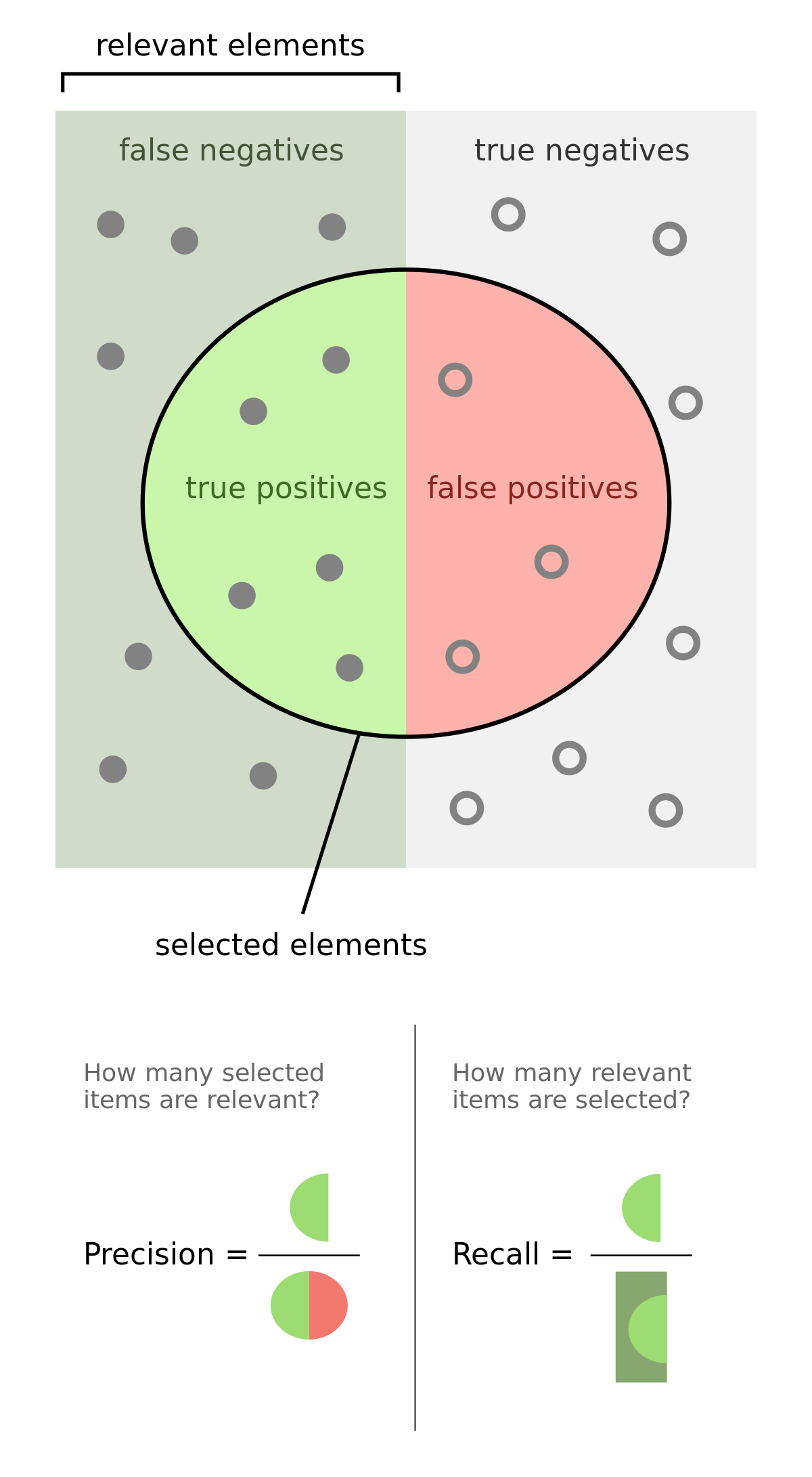
Now, it is time to train and evaluate our model using the F1 score metric. It calculates the weighted average of precision and recall. The higher the F1 score, the more successful the model is. Here is a useful image to understand precision and recall.

Source

Let's start by importing f1_score from the sklearn.metrics library!

from sklearn.metrics import f1_score #used to evaluate the accuracy of a model

Now you may be wondering why do we use the F1 score? The F1 score is an alternative method of predicting the success of a model. It is useful as it investigates false positives and false negatives. In specific real-life scenarios, such as diagnosing cancer, where the distribution of results is unequal, using an F1 score is a more accurate way of judging the performance of a model.

Then, let's create a method that predicts the labels and gives us a specific F1 score and accuracy score after specific features such as x_train and x_test are passed with targets like y_train and y_test.

def label_predict(model, features, target):
   # Makes predictions using Logistic Regression based on accuracy metrics and the F1 score.
    y_prediction = model.predict(features)

    return f1_score(target, y_prediction, pos_label='H')
#returns the F1 score - input parameters are the targets (y_train, and y_test), 
# and the positive label of a home win to ensure the precision and recall calculated is done accurately

Exercise: Return the accuracy score

But we are missing something. We also need to return the accuracy score. Try to write one line of a code that successfully does this.

Hint: You need to find the number of times the target is equal to the prediction.

Solution

acc = sum(target == y_prediction) / float(len(y_prediction))

This takes the sum of the instances where the prediction is the same as the actual output divided by the total number of predictions.

This needs to be added to the label_predict method. Therefore, our method is:

def label_predict(model, features, target):
   # Makes predictions using Logistic Regression based on accuracy metrics and the F1 score.
    y_prediction = model.predict(features)

    return f1_score(target, y_prediction, pos_label='H'), sum(target == y_prediction) / float(len(y_prediction))

Now, we need to create a method that trains the model and outputs the F1 and accuracy score for the training and testing data sets.

def train_predictions(model, x_train, y_train, x_test, y_test):
    # Train the Logistic Regression model
    model.fit(x_train, y_train)
    
   #Outputs metrics for training dataset
    f1, acc = label_predict(model, x_train, y_train)
    print ("The F1 score for the training dataset was "+str(f1))
    print ("The accuracy score for the training dataset was "+str(acc))
   #Outputs metrics for testing dataset
    f1, acc = label_predict(model, x_test, y_test)
    print ("The F1 score for the testing dataset was "+str(f1))
    print ("The accuracy score for the testing dataset was "+str(acc))

Now, we need to actually put a specific model rather than model. sklearn has a Logistic Regression model that needs to be imported. After this, we need to create a variable that stores this model.

from sklearn.linear_model import LogisticRegression #used to carry out Logistic Regression
LR = LogisticRegression(random_state = 4) 
#creates a LR model. random state is used to shuffle the data

train_predictions(LR, x_train, y_train, x_test, y_test)
#finally we call the method we created with the Logistic Regression model

Our metric output is the following:

The F1 score for the training dataset was 0.6202690582959641
The accuracy score for the training dataset was 0.663968253968254
The F1 score for the testing dataset was 0.6443381180223285
The accuracy score for the testing dataset was 0.6814285714285714

This suggests that the training dataset had an F1 score of approximately 62% and 66% accuracy. More importantly, our testing dataset had an F1 score of around 64%, while the accuracy was a little over 68%.

Not bad for our first attempt!

Summary and Improvements

There you go! That is how you create a model that is able to predict if the home team will win or not. Evidently, this isn’t the best model, but that is something that you will encounter while working on creating models. Your first attempt will usually not be the best. There will always be areas to work on and improve, such as trying different techniques such as using Support Vector Machines.